타이타닉 생존여부 확인 by 로지스틱 회귀모델
로지스틱 회귀모델을 이용해서 타이타닉호 승선객의 생존여부 확인하기
age 결측치 값은 다음과 같이 처리
- 생존자(survived = 1 )는 생존자 나이의 평균으로 대체
- 생존자(survived = 0 )는 사망자 나이의 평균으로 대체
import pandas as pd
import numpy as np
import statsmodels.api as sm
import matplotlib.pyplot as plt

from sklearn.linear_model import LogisticRegression
from sklearn.model_selection import train_test_split
from sklearn import metrics
from sklearn.metrics import confusion_matrix
from sklearn.metrics import accuracy_score, roc_auc_score, roc_curve
titanic = pd.read_csv("train.csv")
titanic.head()
| PassengerId | Survived | Pclass | Name | Sex | Age | SibSp | Parch | Ticket | Fare | Cabin | Embarked | |
|---|---|---|---|---|---|---|---|---|---|---|---|---|
| 0 | 1 | 0 | 3 | Braund, Mr. Owen Harris | male | 22.0 | 1 | 0 | A/5 21171 | 7.2500 | NaN | S |
| 1 | 2 | 1 | 1 | Cumings, Mrs. John Bradley (Florence Briggs Th... | female | 38.0 | 1 | 0 | PC 17599 | 71.2833 | C85 | C |
| 2 | 3 | 1 | 3 | Heikkinen, Miss. Laina | female | 26.0 | 0 | 0 | STON/O2. 3101282 | 7.9250 | NaN | S |
| 3 | 4 | 1 | 1 | Futrelle, Mrs. Jacques Heath (Lily May Peel) | female | 35.0 | 1 | 0 | 113803 | 53.1000 | C123 | S |
| 4 | 5 | 0 | 3 | Allen, Mr. William Henry | male | 35.0 | 0 | 0 | 373450 | 8.0500 | NaN | S |
titanic.info()
<class 'pandas.core.frame.DataFrame'>
RangeIndex: 891 entries, 0 to 890
Data columns (total 12 columns):
 #   Column       Non-Null Count  Dtype
---  ------       --------------  -----
 0   PassengerId  891 non-null    int64
 1   Survived     891 non-null    int64
 2   Pclass       891 non-null    int64
 3   Name         891 non-null    object
 4   Sex          891 non-null    object
 5   Age          714 non-null    float64
 6   SibSp        891 non-null    int64
 7   Parch        891 non-null    int64
 8   Ticket       891 non-null    object
 9   Fare         891 non-null    float64
 10  Cabin        204 non-null    object
 11  Embarked     889 non-null    object
dtypes: float64(2), int64(5), object(5)
memory usage: 83.7+ KB
titanic.describe()
| PassengerId | Survived | Pclass | Age | SibSp | Parch | Fare | |
|---|---|---|---|---|---|---|---|
| count | 891.000000 | 891.000000 | 891.000000 | 714.000000 | 891.000000 | 891.000000 | 891.000000 |
| mean | 446.000000 | 0.383838 | 2.308642 | 29.699118 | 0.523008 | 0.381594 | 32.204208 |
| std | 257.353842 | 0.486592 | 0.836071 | 14.526497 | 1.102743 | 0.806057 | 49.693429 |
| min | 1.000000 | 0.000000 | 1.000000 | 0.420000 | 0.000000 | 0.000000 | 0.000000 |
| 25% | 223.500000 | 0.000000 | 2.000000 | 20.125000 | 0.000000 | 0.000000 | 7.910400 |
| 50% | 446.000000 | 0.000000 | 3.000000 | 28.000000 | 0.000000 | 0.000000 | 14.454200 |
| 75% | 668.500000 | 1.000000 | 3.000000 | 38.000000 | 1.000000 | 0.000000 | 31.000000 |
| max | 891.000000 | 1.000000 | 3.000000 | 80.000000 | 8.000000 | 6.000000 | 512.329200 |
#변수제거
titanic_cln = titanic.drop(["PassengerId","Name","Ticket","Cabin"],axis=1)
titanic_cln.head()
| Survived | Pclass | Sex | Age | SibSp | Parch | Fare | Embarked | |
|---|---|---|---|---|---|---|---|---|
| 0 | 0 | 3 | male | 22.0 | 1 | 0 | 7.2500 | S |
| 1 | 1 | 1 | female | 38.0 | 1 | 0 | 71.2833 | C |
| 2 | 1 | 3 | female | 26.0 | 0 | 0 | 7.9250 | S |
| 3 | 1 | 1 | female | 35.0 | 1 | 0 | 53.1000 | S |
| 4 | 0 | 3 | male | 35.0 | 0 | 0 | 8.0500 | S |
titanic_cln.info()
<class 'pandas.core.frame.DataFrame'>
RangeIndex: 891 entries, 0 to 890
Data columns (total 8 columns):
 #   Column    Non-Null Count  Dtype
---  ------    --------------  -----
 0   Survived  891 non-null    int64
 1   Pclass    891 non-null    int64
 2   Sex       891 non-null    object
 3   Age       714 non-null    float64
 4   SibSp     891 non-null    int64
 5   Parch     891 non-null    int64
 6   Fare      891 non-null    float64
 7   Embarked  889 non-null    object
dtypes: float64(2), int64(4), object(2)
memory usage: 55.8+ KB
#결측치 처리

#생존자 나이 평균
sur1_mean = titanic_cln[titanic_cln["Survived"]==1]["Age"].mean()

#사망자 나이 평균
sur0_mean = titanic_cln[titanic_cln["Survived"]==0]["Age"].mean()

print(sur1_mean, sur0_mean)
28.343689655172415 30.62617924528302
titanic_cln[titanic_cln["Survived"]==1]["Age"].fillna(sur1_mean)
titanic_cln[titanic_cln["Survived"]==0]["Age"].fillna(sur0_mean)
0      22.000000
4      35.000000
5      30.626179
6      54.000000
7       2.000000
         ...
884    25.000000
885    39.000000
886    27.000000
888    30.626179
890    32.000000
Name: Age, Length: 549, dtype: float64
#결측치 처리는 loc로
titanic_cln.loc[titanic_cln["Survived"]==1,"Age"] = titanic_cln[titanic_cln["Survived"]==1]["Age"].fillna(sur1_mean)
titanic_cln.loc[titanic_cln["Survived"]==0,"Age"] = titanic_cln[titanic_cln["Survived"]==0]["Age"].fillna(sur0_mean)
#age 부분 다 채워진거 확인
titanic_cln.info()
<class 'pandas.core.frame.DataFrame'>
RangeIndex: 891 entries, 0 to 890
Data columns (total 8 columns):
 #   Column    Non-Null Count  Dtype
---  ------    --------------  -----
 0   Survived  891 non-null    int64
 1   Pclass    891 non-null    int64
 2   Sex       891 non-null    object
 3   Age       891 non-null    float64
 4   SibSp     891 non-null    int64
 5   Parch     891 non-null    int64
 6   Fare      891 non-null    float64
 7   Embarked  889 non-null    object
dtypes: float64(2), int64(4), object(2)
memory usage: 55.8+ KB
titanic_cln["Embarked"].value_counts()
S    644
C    168
Q     77
Name: Embarked, dtype: int64
print(titanic_cln["Embarked"].value_counts().index[0])
#s가 제일 많으니까 나머지 결측값에도 s를 넣어줄것
S
titanic_cln["Embarked"] = titanic_cln["Embarked"].fillna(titanic_cln["Embarked"].value_counts().index[0])
titanic_cln.info()
<class 'pandas.core.frame.DataFrame'>
RangeIndex: 891 entries, 0 to 890
Data columns (total 8 columns):
 #   Column    Non-Null Count  Dtype
---  ------    --------------  -----
 0   Survived  891 non-null    int64
 1   Pclass    891 non-null    int64
 2   Sex       891 non-null    object
 3   Age       891 non-null    float64
 4   SibSp     891 non-null    int64
 5   Parch     891 non-null    int64
 6   Fare      891 non-null    float64
 7   Embarked  891 non-null    object
dtypes: float64(2), int64(4), object(2)
memory usage: 55.8+ KB
print(titanic_cln["Pclass"].value_counts())
print(titanic_cln["Sex"].value_counts())
print(titanic_cln["Embarked"].value_counts())
3    491
1    216
2    184
Name: Pclass, dtype: int64
0    577
1    314
Name: Sex, dtype: int64
S    646
C    168
Q     77
Name: Embarked, dtype: int64
#Pclass, sex, Emabarked 변수 타입 변환
#sex 를 female -> 1 male -> 0 으로 변환
titanic_cln["Sex"] = titanic_cln["Sex"].replace(["female","male"],[1,0])
titanic_cln.head()
#sex 변수 변환됨
| Survived | Pclass | Sex | Age | SibSp | Parch | Fare | Embarked | |
|---|---|---|---|---|---|---|---|---|
| 0 | 0 | 3 | 0 | 22.0 | 1 | 0 | 7.2500 | S |
| 1 | 1 | 1 | 1 | 38.0 | 1 | 0 | 71.2833 | C |
| 2 | 1 | 3 | 1 | 26.0 | 0 | 0 | 7.9250 | S |
| 3 | 1 | 1 | 1 | 35.0 | 1 | 0 | 53.1000 | S |
| 4 | 0 | 3 | 0 | 35.0 | 0 | 0 | 8.0500 | S |
#3개의 카테고리로 만들어줄것
titanic_cln["Pclass"]=titanic_cln["Pclass"].astype("category")
titanic_cln["Embarked"]=titanic_cln["Embarked"].astype("category")
titanic_cln.info()
<class 'pandas.core.frame.DataFrame'>
RangeIndex: 891 entries, 0 to 890
Data columns (total 8 columns):
 #   Column    Non-Null Count  Dtype
---  ------    --------------  -----
 0   Survived  891 non-null    int64
 1   Pclass    891 non-null    category
 2   Sex       891 non-null    int64
 3   Age       891 non-null    float64
 4   SibSp     891 non-null    int64
 5   Parch     891 non-null    int64
 6   Fare      891 non-null    float64
 7   Embarked  891 non-null    category
dtypes: category(2), float64(2), int64(4)
memory usage: 43.9 KB
titanic_cln_dum = pd.get_dummies(titanic_cln)
titanic_cln_dum.head()
| Survived | Sex | Age | SibSp | Parch | Fare | Pclass_1 | Pclass_2 | Pclass_3 | Embarked_C | Embarked_Q | Embarked_S | |
|---|---|---|---|---|---|---|---|---|---|---|---|---|
| 0 | 0 | 0 | 22.0 | 1 | 0 | 7.2500 | 0 | 0 | 1 | 0 | 0 | 1 |
| 1 | 1 | 1 | 38.0 | 1 | 0 | 71.2833 | 1 | 0 | 0 | 1 | 0 | 0 |
| 2 | 1 | 1 | 26.0 | 0 | 0 | 7.9250 | 0 | 0 | 1 | 0 | 0 | 1 |
| 3 | 1 | 1 | 35.0 | 1 | 0 | 53.1000 | 1 | 0 | 0 | 0 | 0 | 1 |
| 4 | 0 | 0 | 35.0 | 0 | 0 | 8.0500 | 0 | 0 | 1 | 0 | 0 | 1 |
titanic_cln_dum = sm.add_constant(titanic_cln_dum, has_constant="add")
titanic_cln_dum.head()
| const | const | Survived | Sex | Age | SibSp | Parch | Fare | Pclass_1 | Pclass_2 | Pclass_3 | Embarked_C | Embarked_Q | Embarked_S | |
|---|---|---|---|---|---|---|---|---|---|---|---|---|---|---|
| 0 | 1.0 | 1.0 | 0 | 0 | 22.0 | 1 | 0 | 7.2500 | 0 | 0 | 1 | 0 | 0 | 1 |
| 1 | 1.0 | 1.0 | 1 | 1 | 38.0 | 1 | 0 | 71.2833 | 1 | 0 | 0 | 1 | 0 | 0 |
| 2 | 1.0 | 1.0 | 1 | 1 | 26.0 | 0 | 0 | 7.9250 | 0 | 0 | 1 | 0 | 0 | 1 |
| 3 | 1.0 | 1.0 | 1 | 1 | 35.0 | 1 | 0 | 53.1000 | 1 | 0 | 0 | 0 | 0 | 1 |
| 4 | 1.0 | 1.0 | 0 | 0 | 35.0 | 0 | 0 | 8.0500 | 0 | 0 | 1 | 0 | 0 | 1 |
feature_columns = list(titanic_cln_dum.columns.difference(["Survived"]))


X = titanic_cln_dum[feature_columns]
y = titanic_cln_dum["Survived"]
x_train, x_test, y_train, y_test = train_test_split(X,y,
                                                   train_size=0.7, test_size =0.3,
                                                   random_state=102)
print(x_train.shape, x_test.shape, y_train.shape, y_test.shape)
(623, 13) (268, 13) (623,) (268,)
model = sm.Logit(y_train, x_train)
results = model.fit(method="newton")
Optimization terminated successfully.
         Current function value: 0.441385
         Iterations 7
results.summary()
| Dep. Variable: | Survived | No. Observations: | 623 |
|---|---|---|---|
| Model: | Logit | Df Residuals: | 613 |
| Method: | MLE | Df Model: | 9 |
| Date: | Tue, 26 Jul 2022 | Pseudo R-squ.: | 0.3386 |
| Time: | 15:58:31 | Log-Likelihood: | -274.98 |
| converged: | True | LL-Null: | -415.74 |
| Covariance Type: | nonrobust | LLR p-value: | 2.171e-55 |
| coef | std err | z | P>|z| | [0.025 | 0.975] | |
|---|---|---|---|---|---|---|
| Age | -0.0461 | 0.009 | -4.941 | 0.000 | -0.064 | -0.028 |
| Embarked_C | 0.3284 | 4.11e+07 | 7.99e-09 | 1.000 | -8.06e+07 | 8.06e+07 |
| Embarked_Q | 0.1857 | nan | nan | nan | nan | nan |
| Embarked_S | -0.3197 | nan | nan | nan | nan | nan |
| Fare | 0.0048 | 0.004 | 1.348 | 0.178 | -0.002 | 0.012 |
| Parch | -0.0910 | 0.140 | -0.649 | 0.516 | -0.366 | 0.184 |
| Pclass_1 | 1.0648 | nan | nan | nan | nan | nan |
| Pclass_2 | 0.1762 | nan | nan | nan | nan | nan |
| Pclass_3 | -1.0466 | nan | nan | nan | nan | nan |
| Sex | 2.5486 | 0.239 | 10.675 | 0.000 | 2.081 | 3.017 |
| SibSp | -0.4101 | 0.136 | -3.020 | 0.003 | -0.676 | -0.144 |
| const | 0.1944 | 3.45e+15 | 5.64e-17 | 1.000 | -6.75e+15 | 6.75e+15 |
| const | 0.1944 | 1.25e+15 | 1.56e-16 | 1.000 | -2.44e+15 | 2.44e+15 |
results.params
Age          -0.046104
Embarked_C    0.328389
Embarked_Q    0.185698
Embarked_S   -0.319655
Fare          0.004812
Parch        -0.091043
Pclass_1      1.064840
Pclass_2      0.176165
Pclass_3     -1.046573
Sex           2.548639
SibSp        -0.410117
const         0.194432
const         0.194432
dtype: float64
np.exp(results.params)
#pclass가 1인경우, 생존할 확률이 2배 높음
#변수의 범주가 나뉘지는 경우에는 카테고리로 나눠서 할것
Age            0.954943
Embarked_C     1.388730
Embarked_Q     1.204058
Embarked_S     0.726400
Fare           1.004824
Parch          0.912979
Pclass_1       2.900376
Pclass_2       1.192634
Pclass_3       0.351139
Sex           12.789688
SibSp          0.663573
const          1.214621
const          1.214620
dtype: float64
results.aic
569.9662477300736
y_pred = results.predict(x_test)
y_pred
618    0.868298
849    0.954464
235    0.548751
865    0.715086
731    0.321682
         ...
259    0.627825
760    0.089515
557    0.812292
638    0.358194
504    0.966472
Length: 268, dtype: float64
def PRED(y,threshold):
    Y= y.copy()
    Y[y > threshold] = 1
    Y[y <= threshold] = 0
    return(Y.astype(int))

Y_pred = PRED(y_pred,0.5)
Y_pred
618    1
849    1
235    1
865    1
731    0
      ..
259    1
760    0
557    1
638    0
504    1
Length: 268, dtype: int64
cfmat = confusion_matrix(y_test, Y_pred)
print(cfmat)
[[141  26]
 [ 26  75]]
def acc(cfmat):
    acc =(cfmat[0,0]+cfmat[1,1]/np.sum(cfmat))
    return(acc)

acc(cfmat)
141.27985074626866
threshold = np.arange(0,1,0.1)
table = pd.DataFrame(columns=["ACC"])

for i in threshold:
    Y_pred = PRED(y_pred,i)
    cfmat= confusion_matrix(y_test, Y_pred)
    table.loc[i] = acc(cfmat)

table.index.name="threshold"
table.columns.name="performance"
table

#0.6일때 정확도가 가장 높아짐
| performance | ACC |
|---|---|
| threshold | |
| 0.0 | 0.376866 |
| 0.1 | 52.358209 |
| 0.2 | 105.332090 |
| 0.3 | 121.313433 |
| 0.4 | 135.294776 |
| 0.5 | 141.279851 |
| 0.6 | 149.257463 |
| 0.7 | 161.190299 |
| 0.8 | 164.134328 |
| 0.9 | 166.082090 |
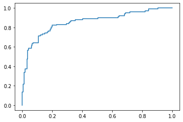
fpr, tpr, thresholds = metrics.roc_curve(y_test,y_pred, pos_label=1)
plt.plot(fpr,tpr)

auc=np.trapz(tpr,fpr)
print("AUC: ",auc)
AUC: 0.859370368174542
회귀계수 축소모형을 이용해서 타이타닉호 승선객의 생존여부 확인
from sklearn.linear_model import Ridge,Lasso,ElasticNet
lasso = Lasso(alpha = 0.01)
lasso.fit(x_train,y_train)
Lasso(alpha=0.01)
lasso.coef_
array([-0.00602402,  0.        ,  0.        , -0.05284511,  0.00103671,
       -0.00212009,  0.08610017, -0.        , -0.16710225,  0.42002796,
       -0.04601298,  0.        ,  0.        ])
pred_y_lasso = lasso.predict(x_test)
pred_Y_lasso = PRED(pred_y_lasso, 0.5)
cfmat = confusion_matrix(y_test, pred_Y_lasso)
print(acc(cfmat))
145.26865671641792
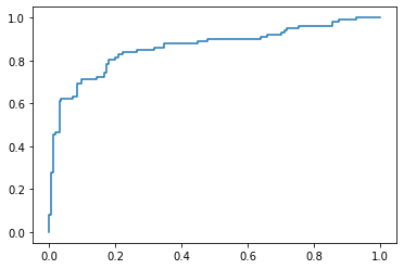
fpr, tpr, thresholds = metrics.roc_curve(y_test, pred_y_lasso)
plt.plot(fpr,tpr)

auc=np.trapz(tpr,fpr)
print("AUC: ", auc)
AUC: 0.862571885931108
threshold = np.arange(0,1,0.1)
table = pd.DataFrame(columns = ["ACC"])

for i in threshold:
    Y_pred = PRED(pred_y_lasso, i)
    cfmat = confusion_matrix(y_test, Y_pred)
    table.loc[i]=acc(cfmat)


table.index.name = "threshold"
table.columns.name="performance"
table
| performance | ACC |
|---|---|
| threshold | |
| 0.0 | 2.376866 |
| 0.1 | 21.373134 |
| 0.2 | 93.332090 |
| 0.3 | 116.320896 |
| 0.4 | 137.298507 |
| 0.5 | 145.268657 |
| 0.6 | 161.235075 |
| 0.7 | 165.145522 |
| 0.8 | 166.097015 |
| 0.9 | 166.041045 |
alpha = np.logspace(-3,1,5)
alpha
array([1.e-03, 1.e-02, 1.e-01, 1.e+00, 1.e+01])
data = []
acc_table = []


for i,a in enumerate(alpha):
    lasso = Lasso(alpha=a).fit(x_train,y_train)
    data.append(pd.Series(np.hstack([lasso.intercept_, lasso.coef_])))
    y_pred = lasso.predict(x_test)
    y_pred =PRED(y_pred,0.5)
    cfmat = confusion_matrix(y_test,y_pred)
    acc_table.append((acc(cfmat)))


df_lasso = pd.DataFrame(data, index= alpha).T
df_lasso
#라소를 적용한 모형의 회귀계수
| 0.001 | 0.010 | 0.100 | 1.000 | 10.000 | |
|---|---|---|---|---|---|
| 0 | 0.557221 | 0.519114 | 0.414021 | 0.314982 | 0.386838 |
| 1 | -0.006679 | -0.006024 | -0.004045 | -0.000000 | -0.000000 |
| 2 | 0.018281 | 0.000000 | 0.000000 | 0.000000 | 0.000000 |
| 3 | -0.000000 | 0.000000 | 0.000000 | 0.000000 | -0.000000 |
| 4 | -0.077428 | -0.052845 | -0.000000 | -0.000000 | -0.000000 |
| 5 | 0.000619 | 0.001037 | 0.002525 | 0.002147 | 0.000000 |
| 6 | -0.014105 | -0.002120 | -0.000000 | 0.000000 | 0.000000 |
| 7 | 0.140224 | 0.086100 | 0.000000 | 0.000000 | 0.000000 |
| 8 | -0.000000 | -0.000000 | 0.000000 | 0.000000 | 0.000000 |
| 9 | -0.190047 | -0.167102 | -0.000000 | -0.000000 | -0.000000 |
| 10 | 0.458285 | 0.420028 | 0.025301 | 0.000000 | 0.000000 |
| 11 | -0.045830 | -0.046013 | -0.000000 | -0.000000 | -0.000000 |
| 12 | 0.000000 | 0.000000 | 0.000000 | 0.000000 | 0.000000 |
| 13 | 0.000000 | 0.000000 | 0.000000 | 0.000000 | 0.000000 |
acc_table_lasso = pd.DataFrame(acc_table, index= alpha).T
acc_table_lasso
#람다값이 0.01일때 정확도가 제일 높음
| 0.001 | 0.010 | 0.100 | 1.000 | 10.000 | |
|---|---|---|---|---|---|
| 0 | 142.272388 | 145.268657 | 159.059701 | 162.048507 | 167.0 |
Ridge
ridge = Ridge(alpha = 0.01)
ridge.fit(x_train,y_train)
Ridge(alpha=0.01)
ridge.coef_
array([-0.00674968,  0.04090873,  0.01910686, -0.06001559,  0.00057219,
       -0.0154551 ,  0.16156199,  0.01545708, -0.17701907,  0.46253901,
       -0.04580177,  0.        ,  0.        ])
pred_y_ridge = ridge.predict(x_test)
pred_Y_ridge = PRED(pred_y_ridge, 0.5)
cfmat = confusion_matrix(y_test, pred_Y_ridge)
print(acc(cfmat))
142.27611940298507
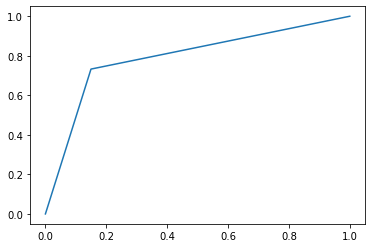
fpr, tpr, thresholds = metrics.roc_curve(y_test, pred_Y_ridge)
plt.plot(fpr,tpr)

auc=np.trapz(tpr,fpr)
print("AUC: ", auc)
AUC: 0.7914863342621689

threshold = np.arange(0,1,0.1)
table = pd.DataFrame(columns = ["ACC"])

for i in threshold:
    Y_pred = PRED(pred_Y_ridge, i)
    cfmat = confusion_matrix(y_test, Y_pred)
    table.loc[i]=acc(cfmat)


table.index.name = "threshold"
table.columns.name="performance"
table
| performance | ACC |
|---|---|
| threshold | |
| 0.0 | 142.276119 |
| 0.1 | 142.276119 |
| 0.2 | 142.276119 |
| 0.3 | 142.276119 |
| 0.4 | 142.276119 |
| 0.5 | 142.276119 |
| 0.6 | 142.276119 |
| 0.7 | 142.276119 |
| 0.8 | 142.276119 |
| 0.9 | 142.276119 |
ElasticNet
elastic = ElasticNet(alpha = 0.1, l1_ratio=0.5)
elastic.fit(x_train,y_train)
ElasticNet(alpha=0.1)
elastic.coef_
array([-0.00401088,  0.        ,  0.        , -0.        ,  0.0023124 ,
       -0.        ,  0.        ,  0.        , -0.00783898,  0.20741403,
       -0.02231027,  0.        ,  0.        ])
pred_y_elastic = elastic.predict(x_test)
pred_Y_elastic = PRED(pred_y_ridge, 0.5)
#0.5 기준으로 1과 0 판단
cfmat = confusion_matrix(y_test, pred_Y_elastic)
print(acc(cfmat))
142.27611940298507
fpr, tpr, thresholds = metrics.roc_curve(y_test, pred_Y_elastic)
plt.plot(fpr,tpr)

auc=np.trapz(tpr,fpr)
print("AUC: ", auc)
AUC: 0.7914863342621689